The Crunch API exposes two ways to consume aggregates from a dataset. The bare Cube API that allows for fine grained and complex aggregation queries and the more modern Aggregations API that uses a concise language to compute analyses.
The Aggregations API speaks the “Dashboard Tile Protocol”, which is part of the Crunch Definitions set of specifications.
Allows to specify an analysis tile and obtain the information straight for rendering requiring little manipulation on the client side (no more cr.cube manipulations needed).
API
The aggregations API can be found inside a dataset under the /api/datasets/:id/aggregate/ URL sending payloads via POST.
The payload is a shoji:view with a value consisting of a list of analysis tiles.
POST /api/datasets/:id/aggregate/

{
  "element": "shoji:view",
  "value": [
	  {...analysis tile...},
	  {...analysis tile...},
  ]
}
And the result will be a 200 Shoji View response containing a list of analysis values for each of the requested tiles in the same order.
HTTP 200 OK

{
  "element": "shoji:view",
  "value": [
	  {...analysis values...},
	  {...analysis values...},
  ]
}
Types of analyses
The analyses are the elements that go inside the list in the payload sent to the endpoint. We support the current list of analyses:
- Frequency: "type": "frequency" - Use this for categorical and multiple response variables.
- Frequency Array: "type": "frequency_array" - Use this to get a 2D table querying a categorical array variable, indicating to use subvariables and categories as rows and columns
- Tabbed frequency array: "type": "tabbed_frequency_array" - Same as the above but allows an extra dimension to be used as tabs
- Crosstab: "type": "crosstab" - For Xtabbing categoricals or multiple response variables, categorical arrays aren’t allowed here, but subvariables of them are.
- Crosstab Array: "type": "crosstab_array"
- Tabbed Crosstab: "type": "tabbed_crosstab" - Allows to specify 3 univariate variables, Multiple response, categorical or subvariables as rows, columns or tabs
- Numeric Summary: "type": "numeric_summary" - For numeric variables only
- Numeric Array Summary: "type": "numeric_array_summary" - For numeric arrays only
Analysis payload
Each analysis consists on an object with the following keys:
{
    "type": "<analysis_type>",  # From the list above
    "cube": {}, // Cube varying on the analysis type,
    "display": {} // Display information including measures,
}
The cube member of the payload will change depending on the type of analysis.
The display information indicates what measures should be provided to render such as percents or counts. To query this endpoint, it is enough to request data as a table.
The cube
The cube bit indicates which of the above analysis types to use. When the <variable target> reference exist it in the following examples, it can refer to a variable alias as a "string" or to a subvariable of an array refered to as an object {"var": "array_alias", "axes": ["subvar_code"]} where array_alias is the alias of the array and subvar_code the code of the subvariable to refer to.
-
Frequency: "type": "frequency"
This operates over categorical or multiple response variables or array subvariables. It only takes the variable that will be used as rows.{ "type": "frequency", "rows": <variable target>, } -
Frequency Array: "type": "frequency_array"
Must indicate the array alias over which the frequency will count. Then must choose the axis to be one of the two for the rows, columns:- {"type": "array_categories"} for the axis to use the categories
- {"axis": "subvariables", "type": "array_axis"} for the axis that uses subvariables
{ "type": "frequency_array", "array": "array_alias", # Categories for rows "rows": {"type": "array_categories"}, # Subvariables for columns "columns": {"type": "array_axis", "axis": "subvariables"}, } -
Tabbed frequency array: "type": "tabbed_frequency_frequency"
Identical to the above, but allows for another univariate reference (cat, mr or subvar) to be used as a third dimention, normally to be rendered as tabs.{ "type": "tabbed_frequency_array", "array": "array_alias", "columns": {"axis": "subvariables", "type": "array_axis"}, "rows": {"type": "array_categories"}, "tabs": <variable target>, } -
Crosstab: "type": "crosstab"
The crosstab takes two univariate references (cat, mr or subvar) and returns a 2-dimensional table for the measures on each intersection. It requires a columns and rows reference.{ "type": "crosstab", "rows": <variable target>, "columns": <variable target>, } -
Crosstab Array: "type": "crosstab_array"
To crosstab an array is similar to its 2-dimensional frequency, but crossed on an extra dimension using tabs.
Can choose the axis to be one of the three for the rows, columns and optional tabs:- <variable target>
- {"type": "array_categories"} for the axis to use the categories
- {"axis": "subvariables", "type": "array_axis"} for the axies that uses subvariables
{ "type": "crosstab_array", "array": "my_ca", "rows": {"type": "array_categories"}, "columns": "wave", "tabs": {"axis": "subvariables", "type": "array_axis"}, } -
Tabbed Crosstab: "type": "tabbed_crosstab"
Constructs a 3-dimensional crosstab of single dimensional references (cat, mr or subvar).{ "type": "tabbed_crosstab", "rows": <variable target>, "columns": <variable target>, "tabs": <variable target>, } -
Numeric Summary: "type": "numeric_summary"
This allows to perform an aggregation over a numeric variable, which must be referenced under aggregation_variable, this can be a single numeric or numeric array subvariable.{ "type": "numeric_summary", "aggregation_variable": <variable target>, } -
Numeric Array Summary: "type": "numeric_array_summary"
Similar to the numeric summary, this one operates over a numeric array. It allows the subdimension {"type": "array_axis", "axis": "subvariables} to be used as a dimension, and to indicate another uni dimensional variable in the other dimension.{ "type": "numeric_array_summary", "aggregation_variable": "NUMARR", "rows": { "type": "array_axis", "axis": "subvariables" }, "columns": <variable target> }
The display
The display field allows to request multiple measures or information about how the analysis will be rendered. For this case table display is enough:
"display": {"type": "table", "measures": ["col_percent"]}
The available measures are:
- col_percent
- row_percent
- percent
- count
- weighted_count
- mean useful for numeric analyses
Example
To connect you’ll need two pieces of information:
- Your API_KEY, can be obtained from the webapp under user settigs
- Your subdomain, the URL to connect, for example yougov.crunch.io
>>> from pycrunch import connect
>>>
>>> site = connect(api_key=API_KEY, site_url="https://<subdomain>.crunch.io/api/")
>>> # Navigate to projects by ID or by name
>>> # project = session.site.projects.by("id")[<project_id>].entity
>>> project = site.projects.by("name")["Parent project"].entity
>>> project = project.by("name")["Child project"].entity
>>> # Then pick your dataset from the project entity.
>>> dataset = project.by("name")["My Dataset"].entity
>>> # Construct the payload with the list of analyses
>>> analyses = [
...    {
...      "type": "cube_analysis",
...      "cube": {"type": "frequency", "rows": "allpets"},
...      "display": {"type": "table", "measures": ["percent"]}
...    },
...    {
...      "type": "cube_analysis",
...      "cube": {"columns": "country", "rows": "favorite_pet", "type": "crosstab"},
...      "display": {"type": "table", "measures": ["col_percent"]}
...    }
... ]
>>> payload = {"element": "shoji:view", "value": analyses}  # Shoji wrapper
>>> response = dataset.aggregate.post(payload).payload
>>> values = response.value
>>> pprint(values)
[{'status': 'ok',
  'values': [{'base_size': [8.0, 8.0, 11.0],
              'labels': {'row': [{'code': 'allpets_cats',
                                  'insertion': False,
                                  'label': 'Cat'},
                                 {'code': 'allpets_dogs',
                                  'insertion': False,
                                  'label': 'Dog'},
                                 {'code': 'allpets_birds',
                                  'insertion': False,
                                  'label': 'Bird'}]},
              'measure': 'percent',
              'shape': [3],
              'values': [50.0, 62.5, 45.45454545454545]}]},
 {'status': 'ok',
  'values': [{'base_size': [[0.0, 3.0, 2.0, 4.0, 4.0],
                            [0.0, 3.0, 2.0, 4.0, 4.0],
                            [0.0, 3.0, 2.0, 4.0, 4.0]],
              'labels': {'col': [{'code': 1,
                                  'insertion': False,
                                  'label': 'Argentina'},
                                 {'code': 2,
                                  'insertion': False,
                                  'label': 'Australia'},
                                 {'code': 3,
                                  'insertion': False,
                                  'label': 'Austria'},
                                 {'code': 4,
                                  'insertion': False,
                                  'label': 'Belgium'},
                                 {'code': 5,
                                  'insertion': False,
                                  'label': 'Brazil'}],
                         'row': [{'code': 1,
                                  'insertion': False,
                                  'label': 'Cat'},
                                 {'code': 2,
                                  'insertion': False,
                                  'label': 'Dog'},
                                 {'code': 3,
                                  'insertion': False,
                                  'label': 'Bird'}]},
              'measure': 'col_percent',
              'shape': [3, 5],
              'values': [['NaN', 100.0, 50.0, 50.0, 0.0],
                         ['NaN', 0.0, 0.0, 25.0, 75.0],
                         ['NaN', 0.0, 50.0, 25.0, 25.0]]}]}]
The response will be a list containing one object per analysis requested.
Each analysis has the result in the values key.
To interpretet the results the values inside each of those objects contains the table to be rendered. The above examples output the following tables:
1-dimensional analysis
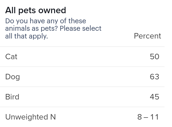
The first analysis is requesting a frequency for the variable allpets in percent which returns this output:
>>> {"type": "frequency", "rows": "allpets"}
{'base_size': [8.0, 8.0, 11.0],
              'labels': {'row': [{'code': 'allpets_cats',
                                  'insertion': False,
                                  'label': 'Cat'},
                                 {'code': 'allpets_dogs',
                                  'insertion': False,
                                  'label': 'Dog'},
                                 {'code': 'allpets_birds',
                                  'insertion': False,
                                  'label': 'Bird'}]},
              'measure': 'percent',
              'shape': [3],
              'values': [50.0, 62.5, 45.45454545454545]}]
To read that output, the values will match the labels one by one
>>> values[0]["values"][0]["values"]
[50.0, 62.5, 45.45454545454545]
>>> values[0]["values"][0]["labels"]
{'row': [{'label': 'Cat', 'insertion': False, 'code': 'allpets_cats'}, {'label': 'Dog', 'insertion': False, 'code': 'allpets_dogs'}, {'label': 'Bird', 'insertion': False, 'code': 'allpets_birds'}]}
>>> values[0]["values"][0]["labels"]["row"]
[{'label': 'Cat', 'insertion': False, 'code': 'allpets_cats'}, {'label': 'Dog', 'insertion': False, 'code': 'allpets_dogs'}, {'label': 'Bird', 'insertion': False, 'code': 'allpets_birds'}]
>>> [l["label"] for l in values[0]["values"][0]["labels"]["row"]]
['Cat', 'Dog', 'Bird']
>>> # Print out the matching row for each label
>>> print("\n".join("%s\t\t%s" % (l["label"], v) for l, v in zip(values[0]["values"][0]["labels"]["row"],  values[0]["values"][0]["values"])))
Cat             50.0
Dog             62.5
Bird            45.45454545454545
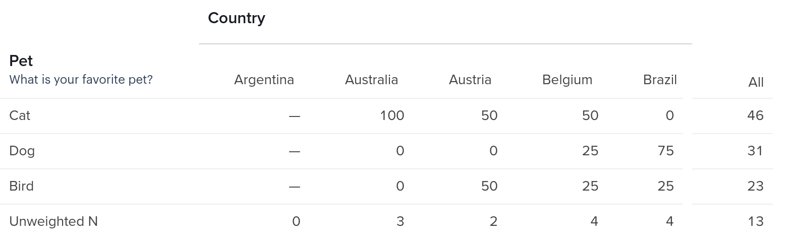
2-dimensional analysis
The second table contains a crosstab for variables country and favorite_pet so the response will not be a single row of values:
[{'base_size': [[0.0, 3.0, 2.0, 4.0, 4.0],
                [0.0, 3.0, 2.0, 4.0, 4.0],
                [0.0, 3.0, 2.0, 4.0, 4.0]],
  'labels': {'col': [{'code': 1, 'insertion': False, 'label': 'Argentina'},
                     {'code': 2, 'insertion': False, 'label': 'Australia'},
                     {'code': 3, 'insertion': False, 'label': 'Austria'},
                     {'code': 4, 'insertion': False, 'label': 'Belgium'},
                     {'code': 5, 'insertion': False, 'label': 'Brazil'}],
             'row': [{'code': 1, 'insertion': False, 'label': 'Cat'},
                     {'code': 2, 'insertion': False, 'label': 'Dog'},
                     {'code': 3, 'insertion': False, 'label': 'Bird'}]},
  'measure': 'col_percent',
  'shape': [3, 5],
  'values': [['NaN', 100.0, 50.0, 50.0, 0.0],
             ['NaN', 0.0, 0.0, 25.0, 75.0],
             ['NaN', 0.0, 50.0, 25.0, 25.0]]}]
The values key here contains the rows of the table, where each list corresponds to a row in the table.
The shape is to be read as [rows, columns]
The labels are ordered and correspond to each of the rows and columns on the values
base_size indicates the denominator used to obtain the percents that these values represent, consider that the measure indicates here col_percents
3-dimensional analyses
A 3 dimensional analyses work the same as 2 dimensional ones, but will be presented as a list of 2 dimensional analyses.
The shape should be read as [rows, columns, tabs] dimensionality. The tabs indicates the size of the first list under values and inside that list, each element corresponds of a 2-dimensional analysis all of shape rows x columns